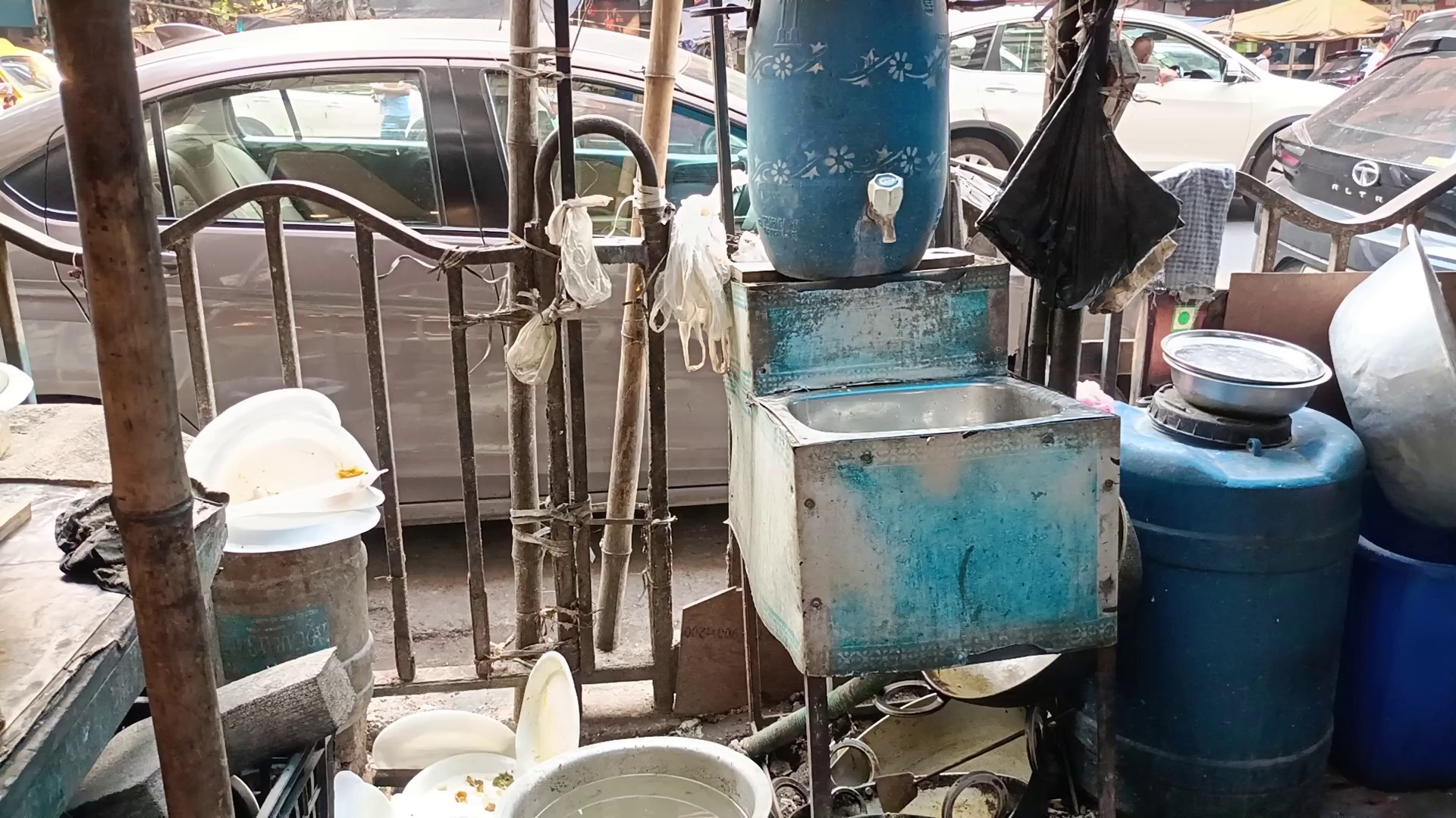
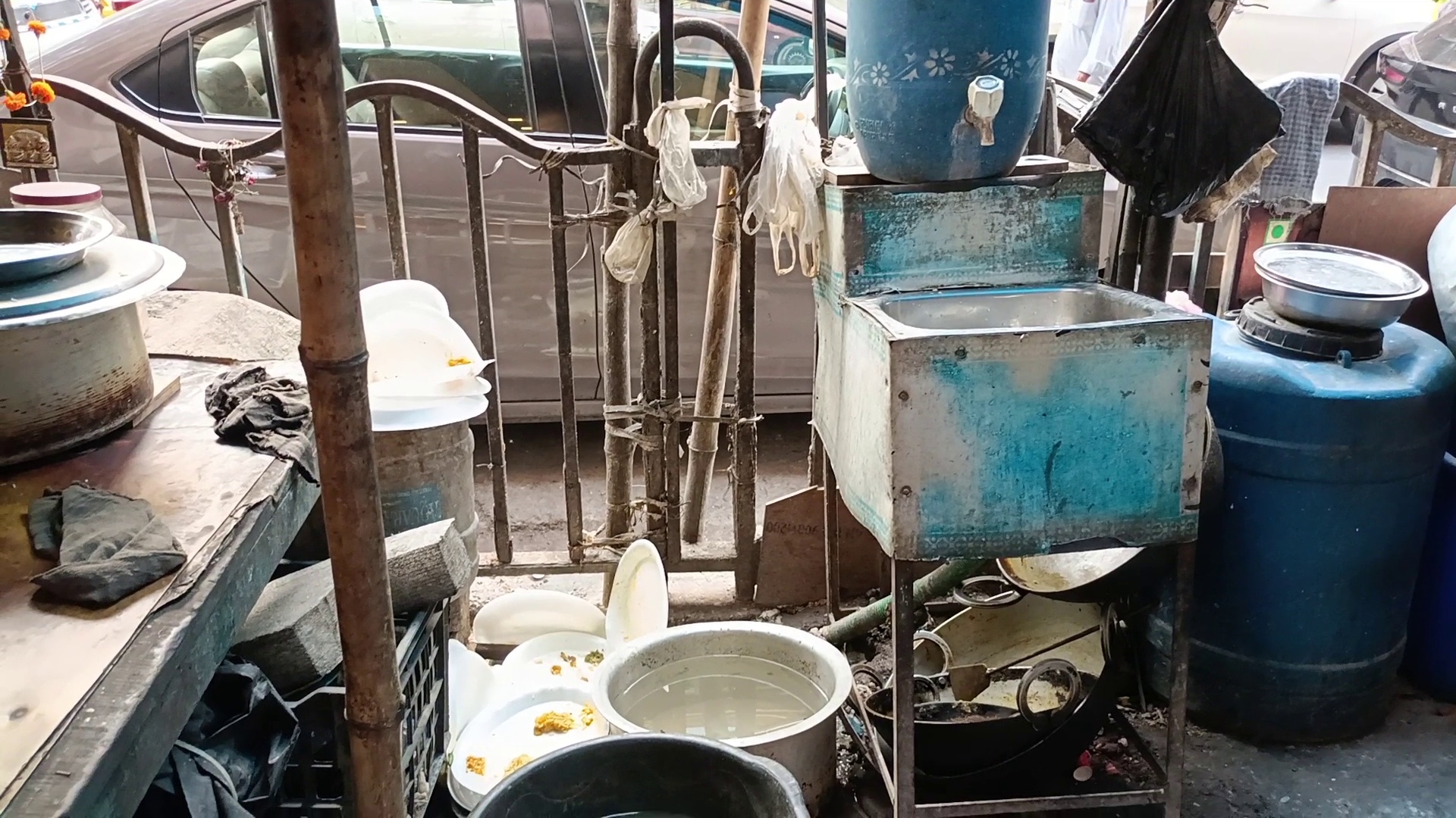
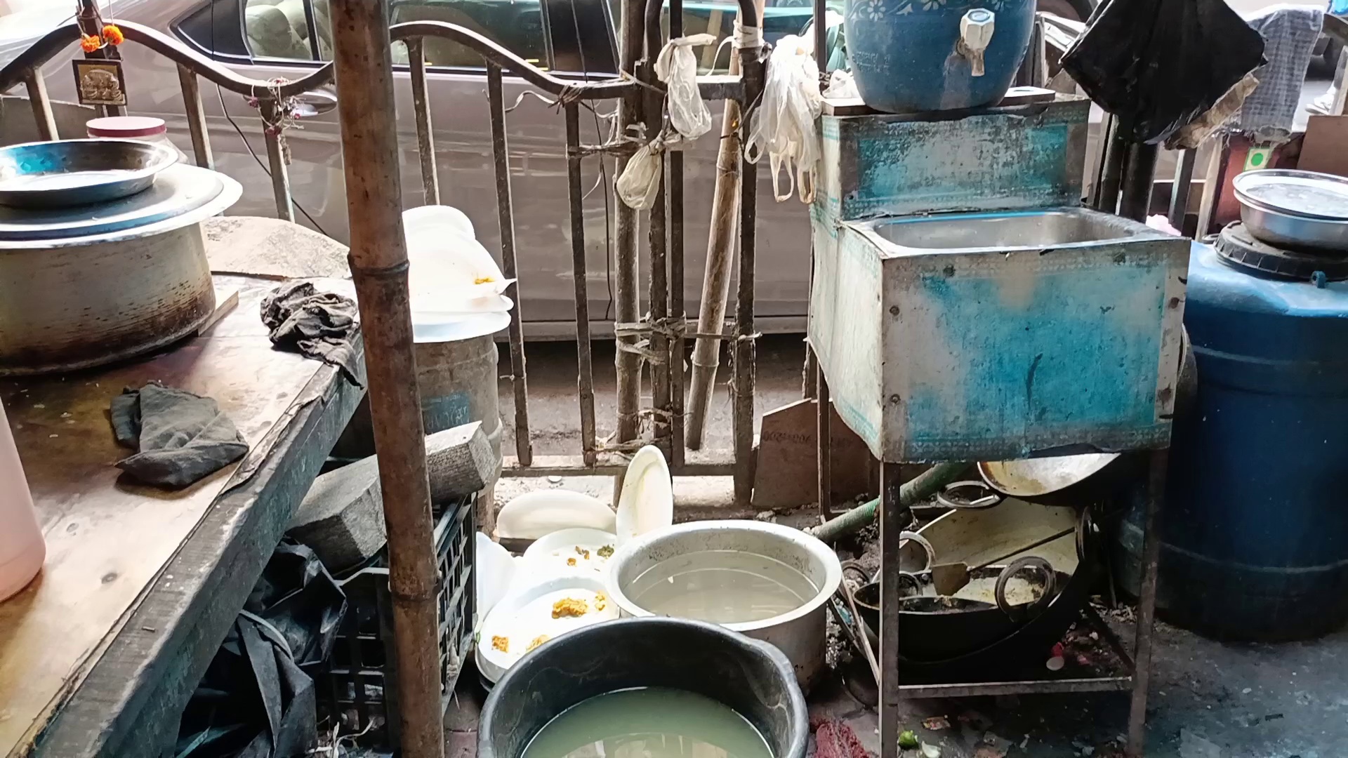
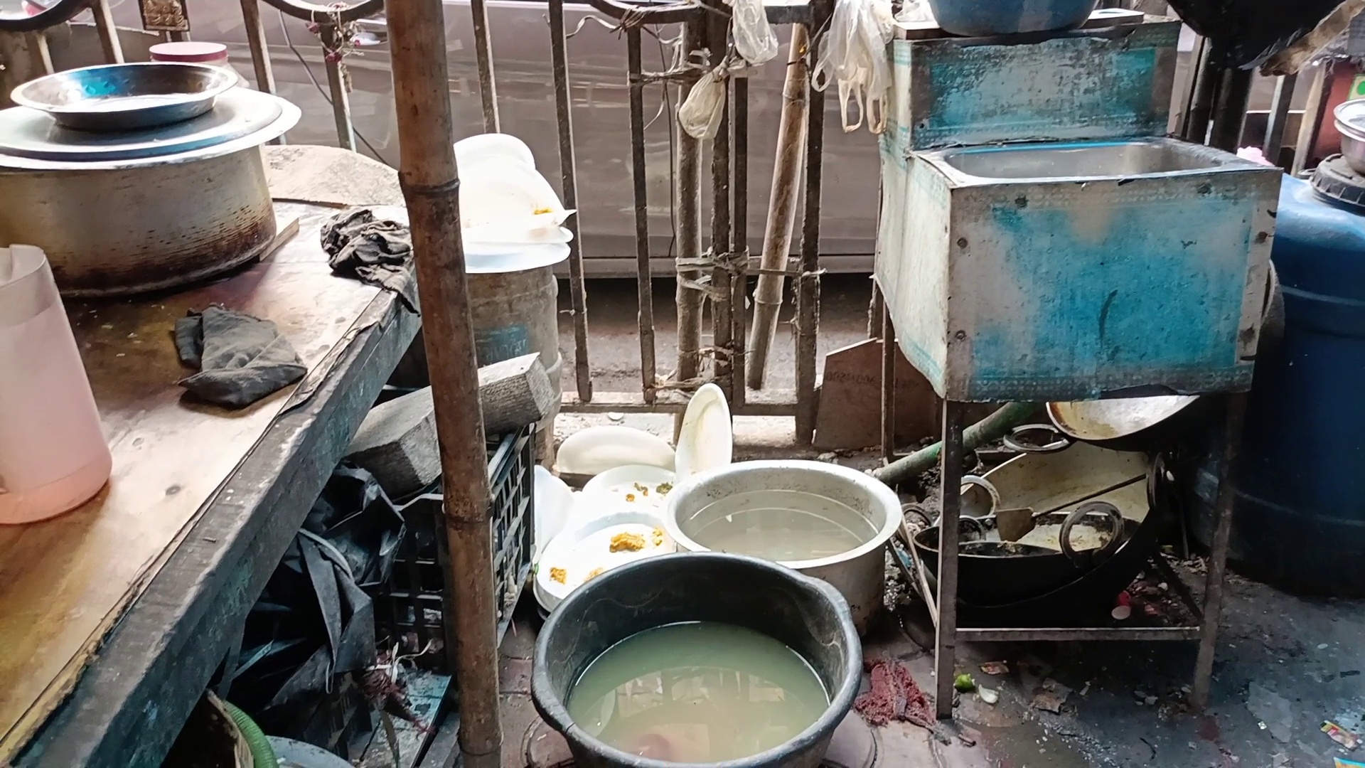
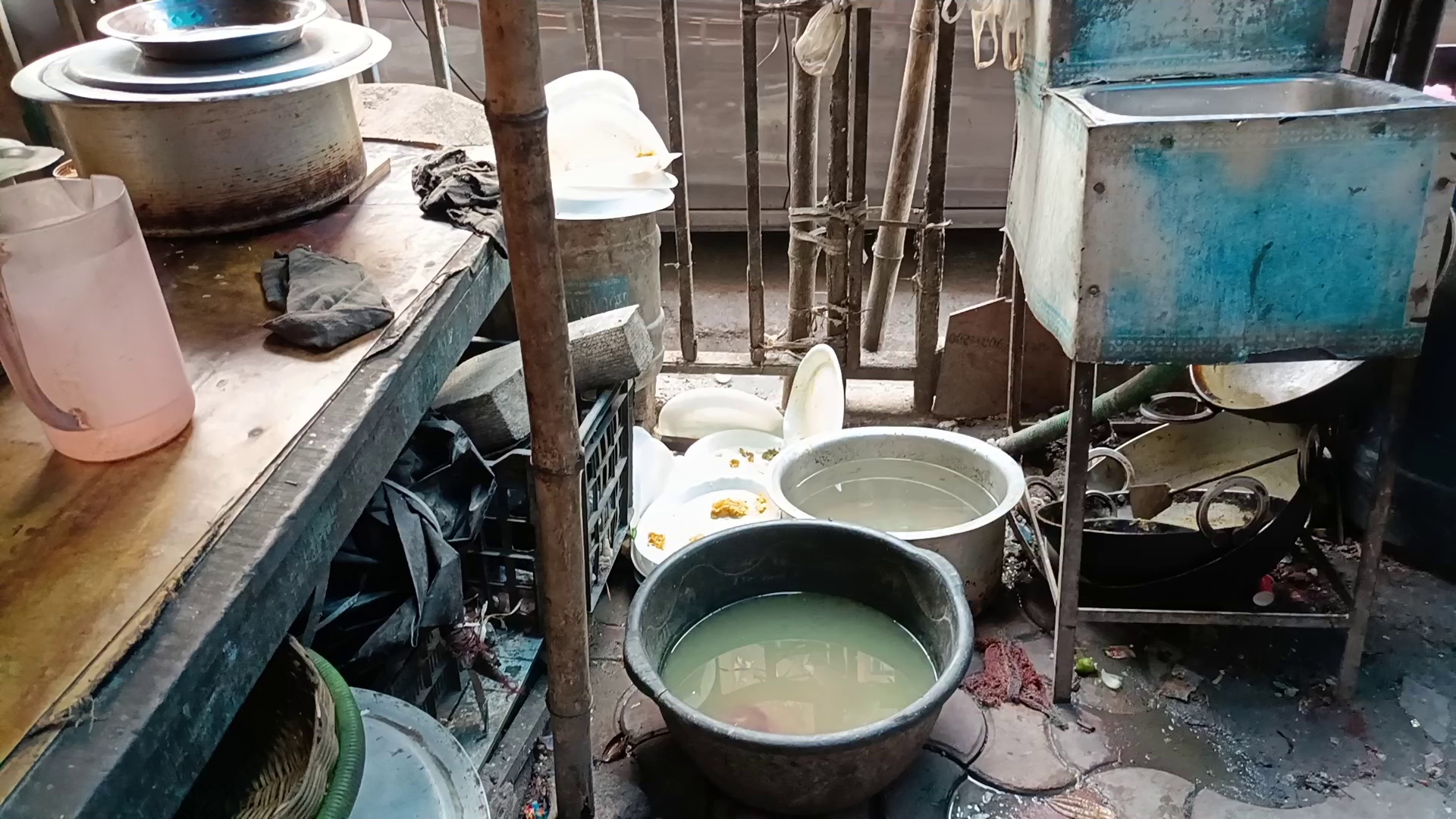
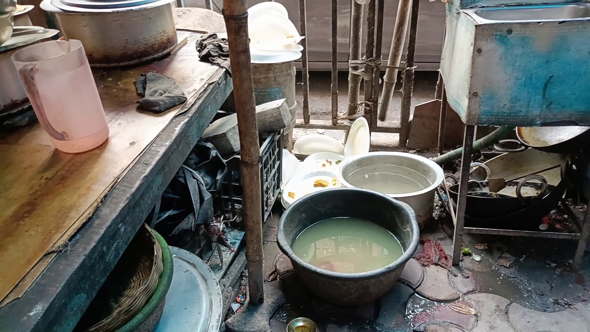
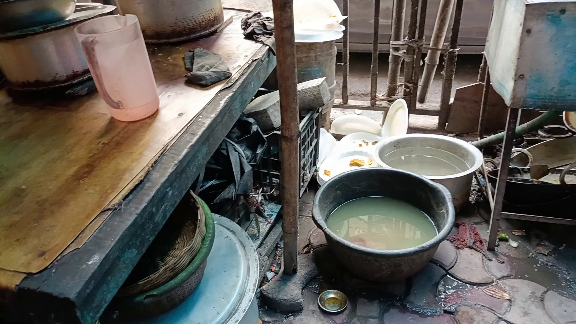
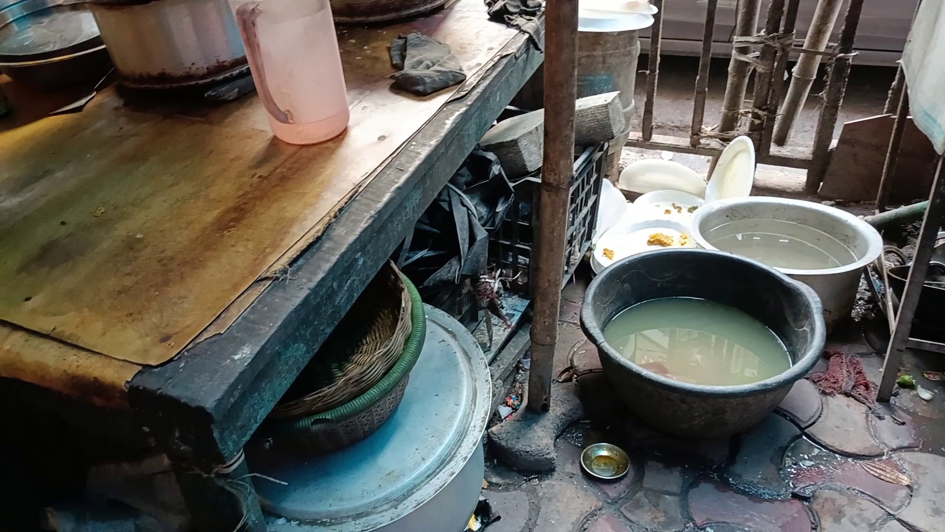
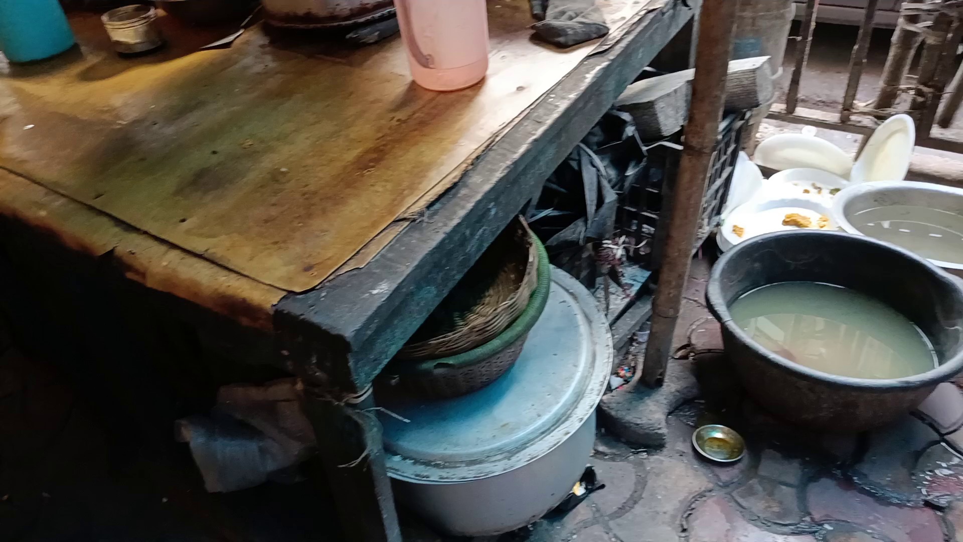
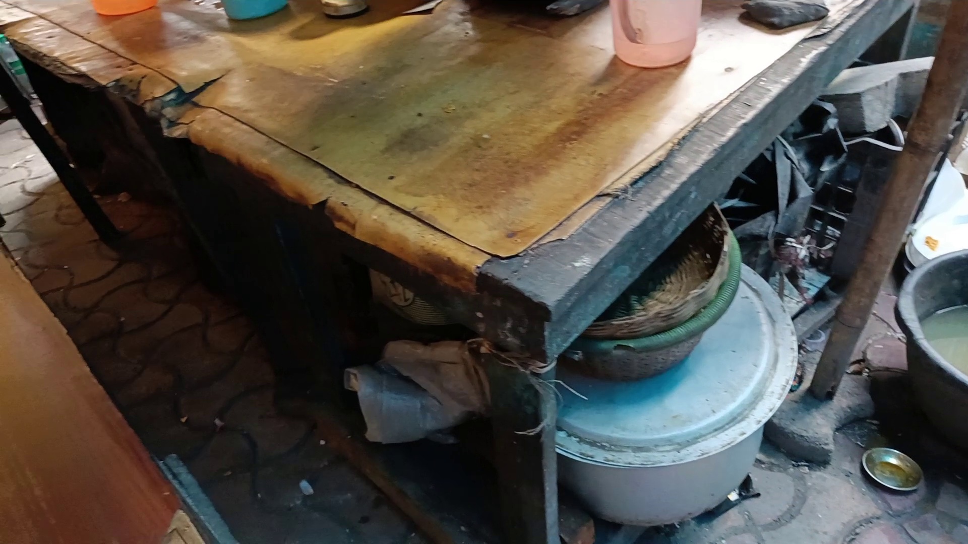
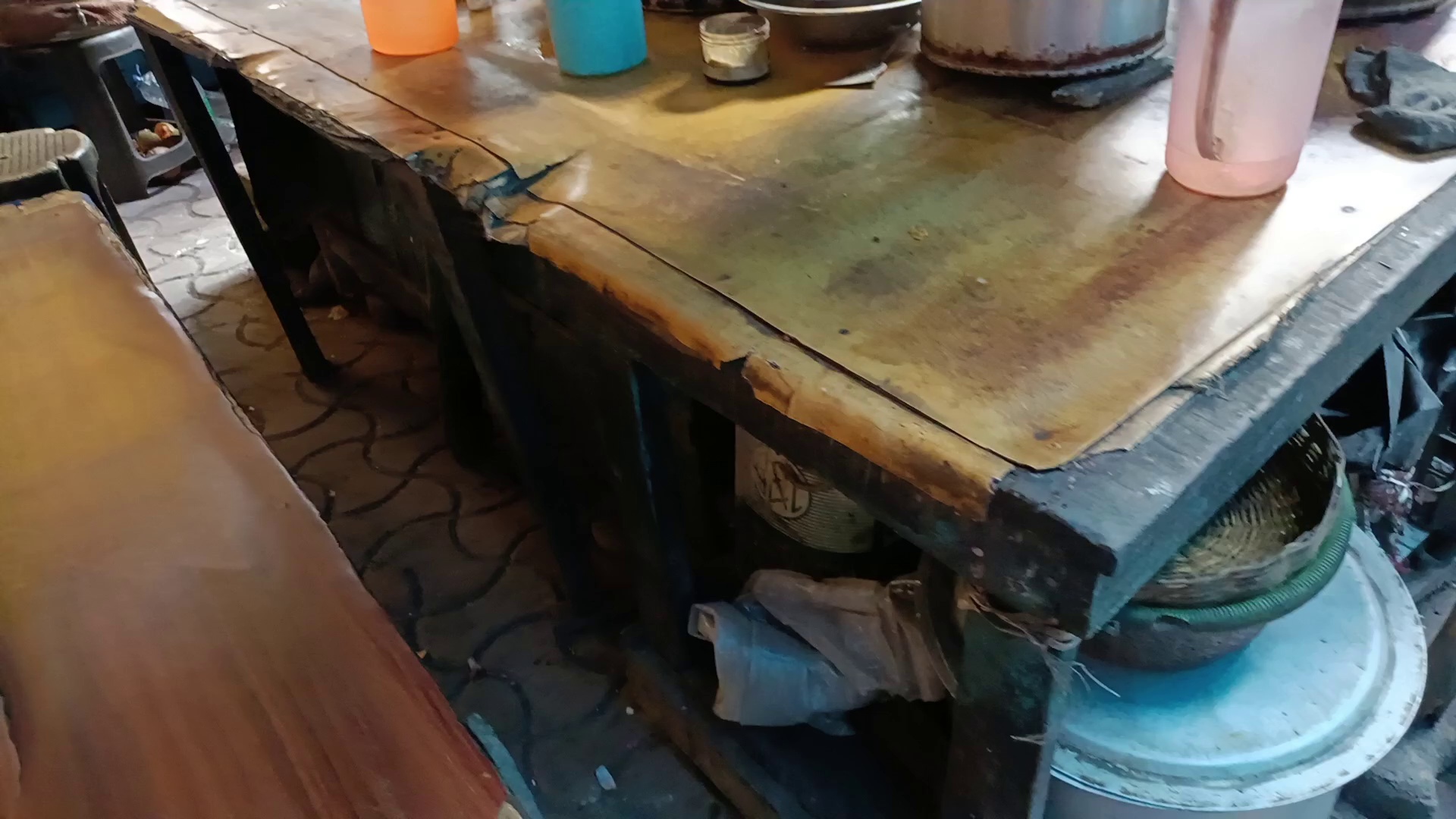
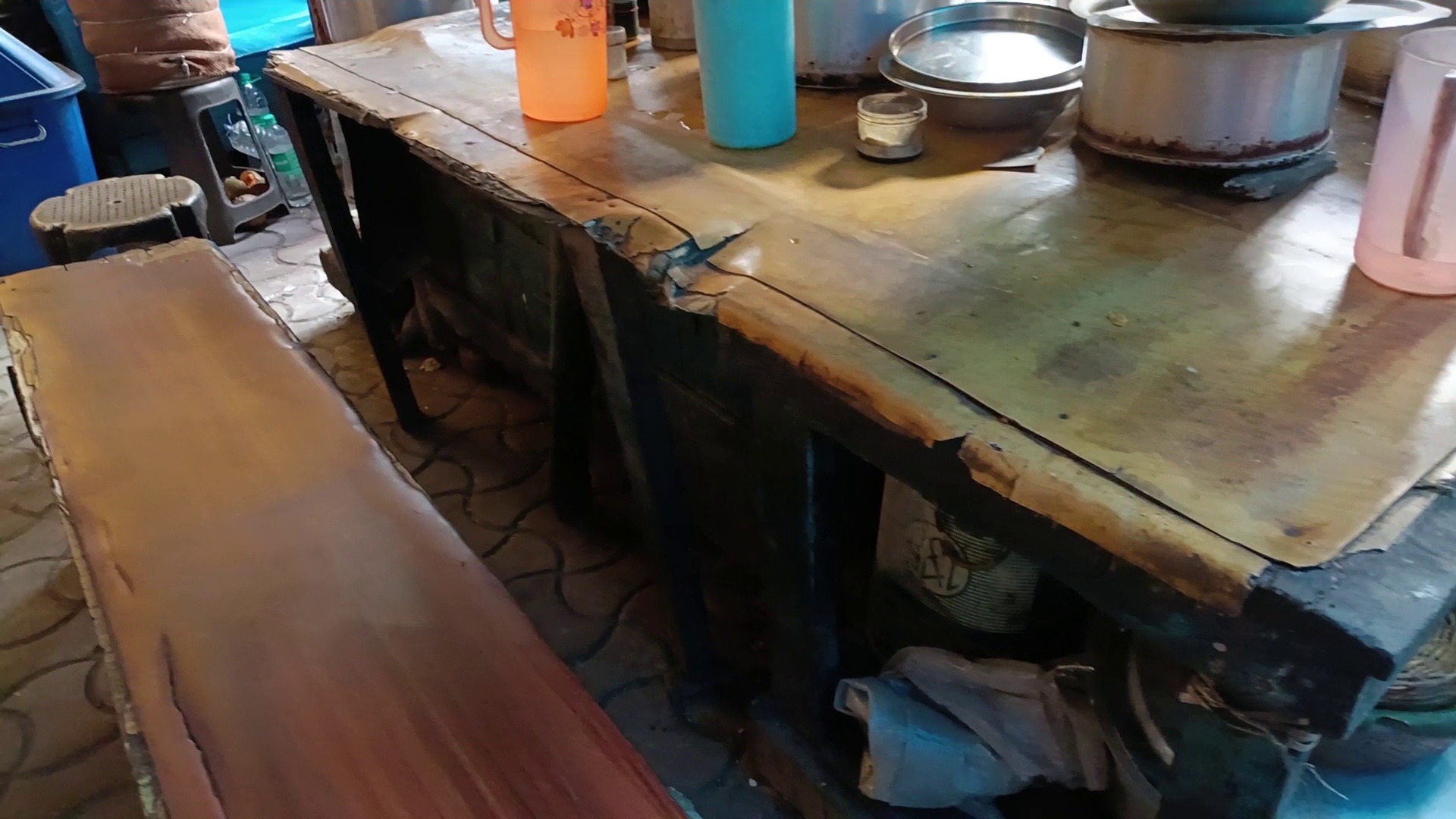
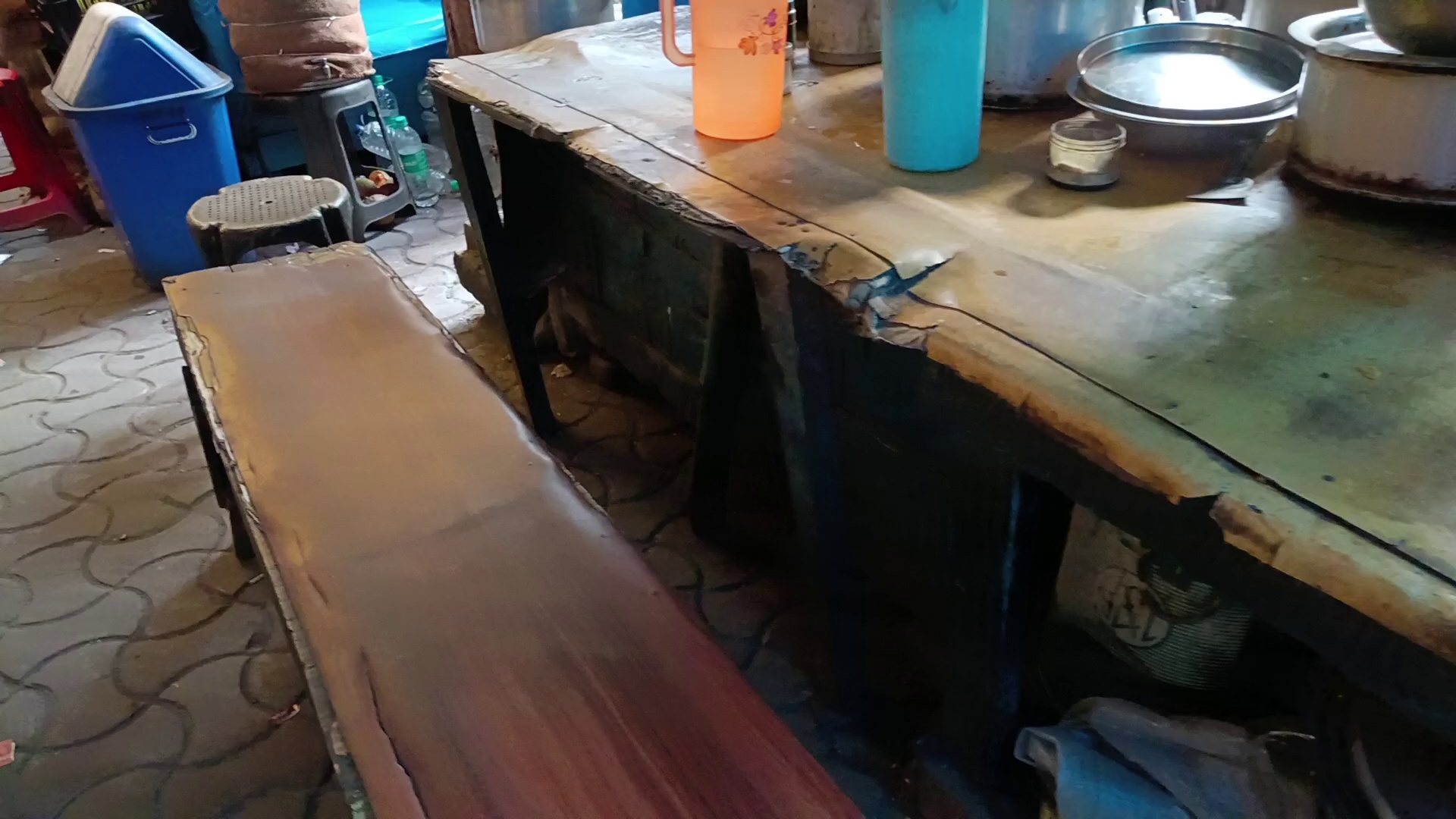

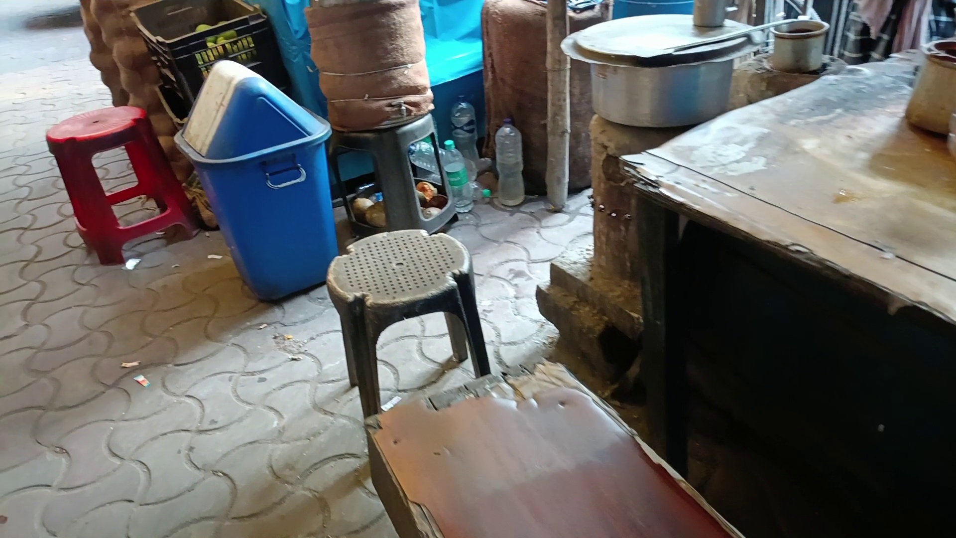
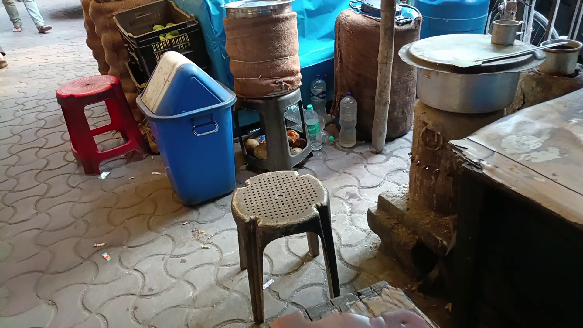
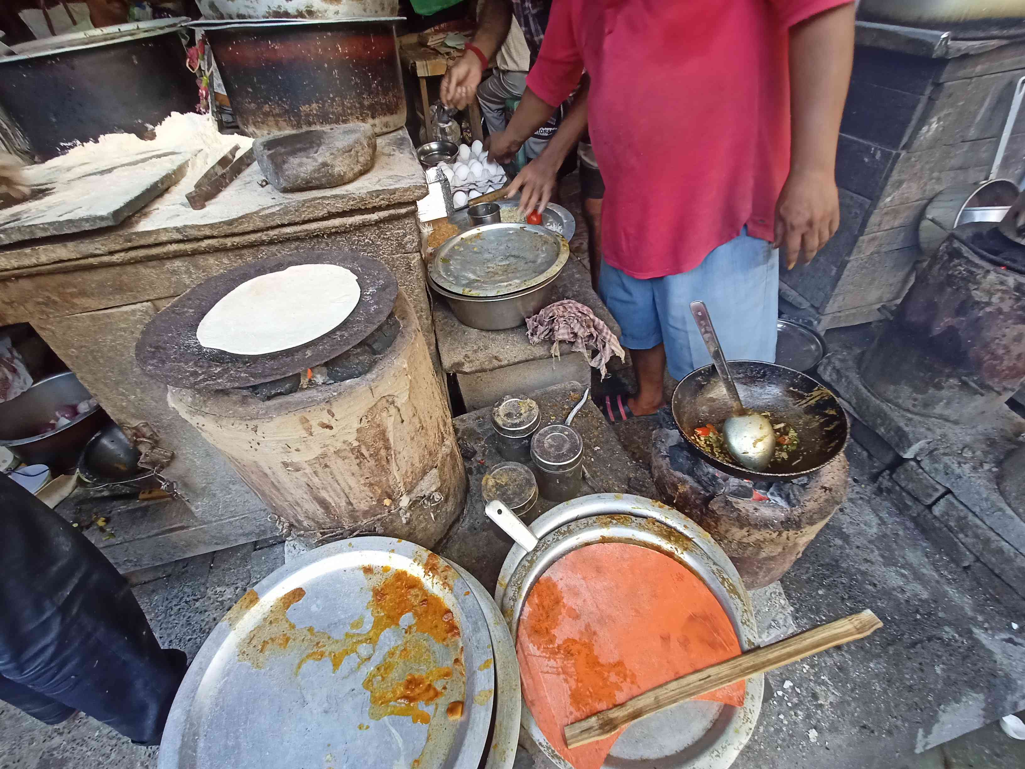
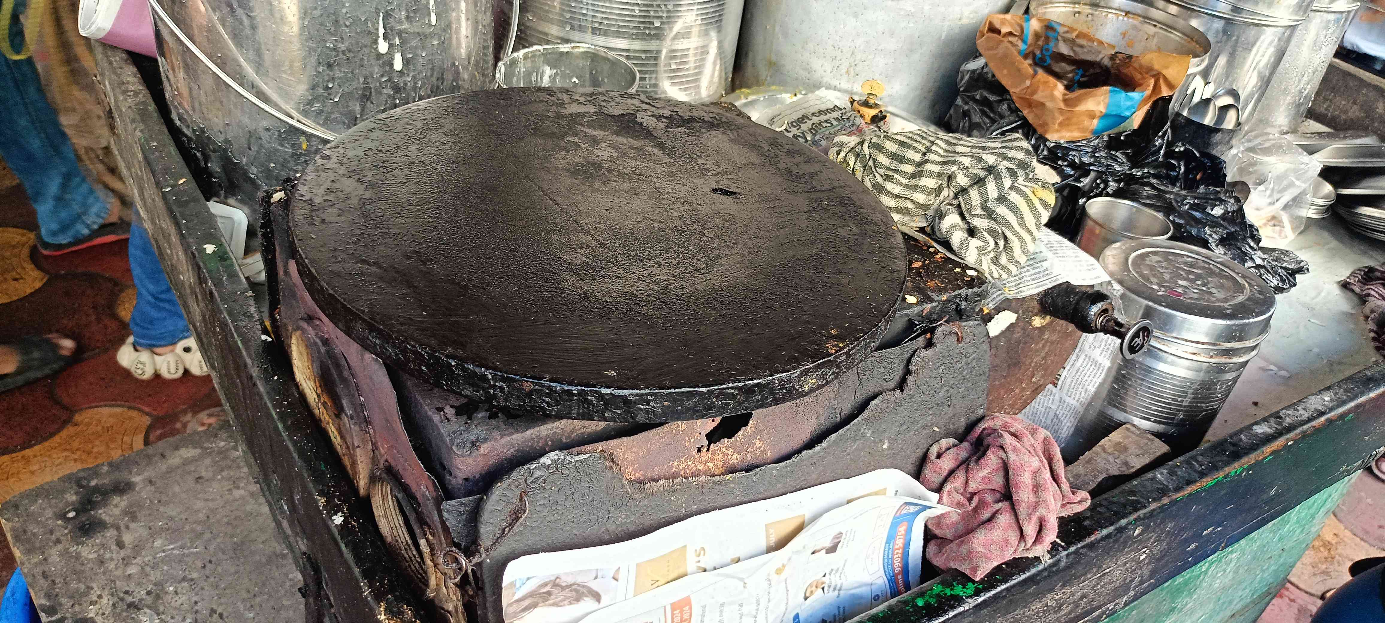
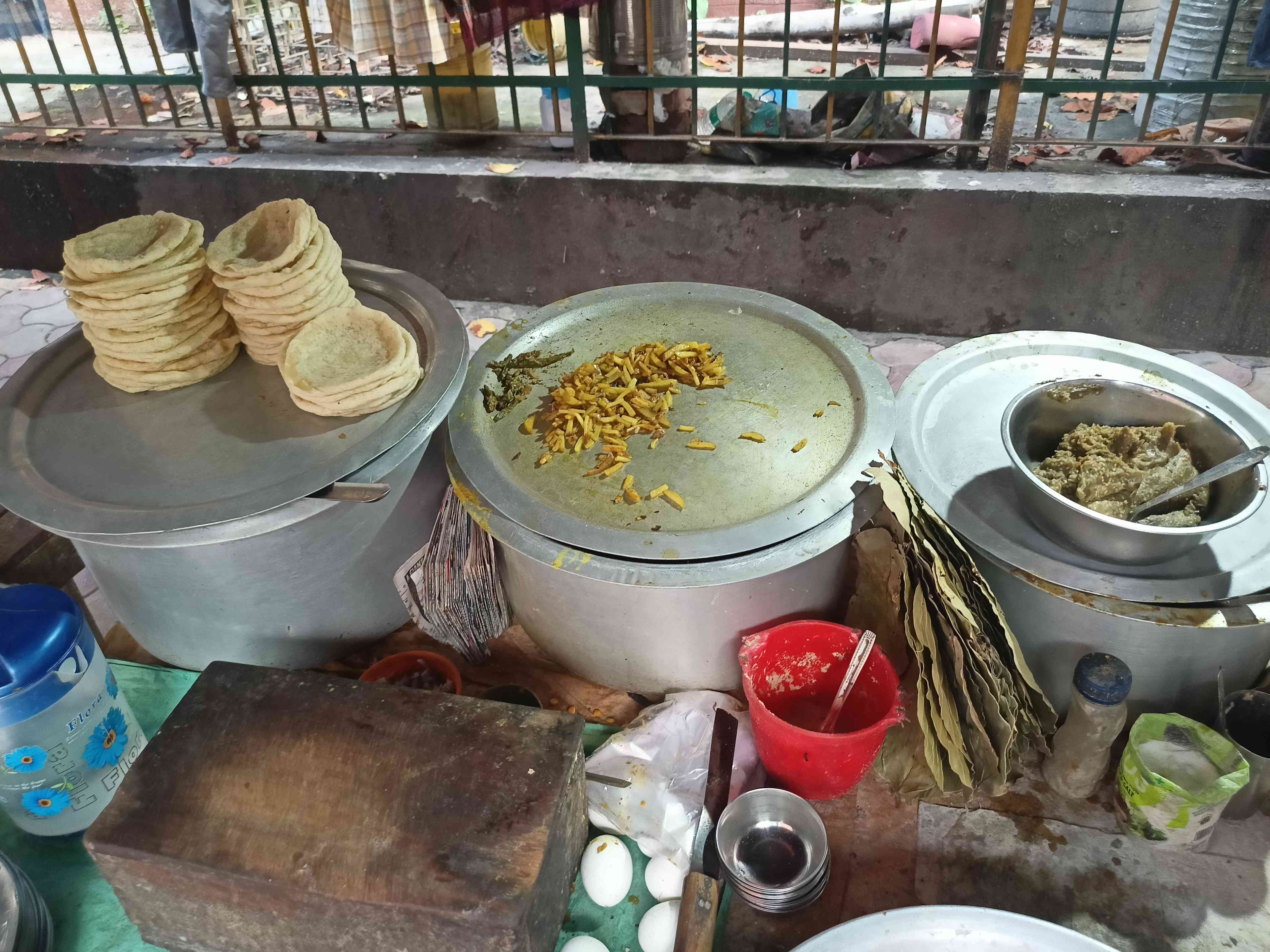
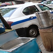
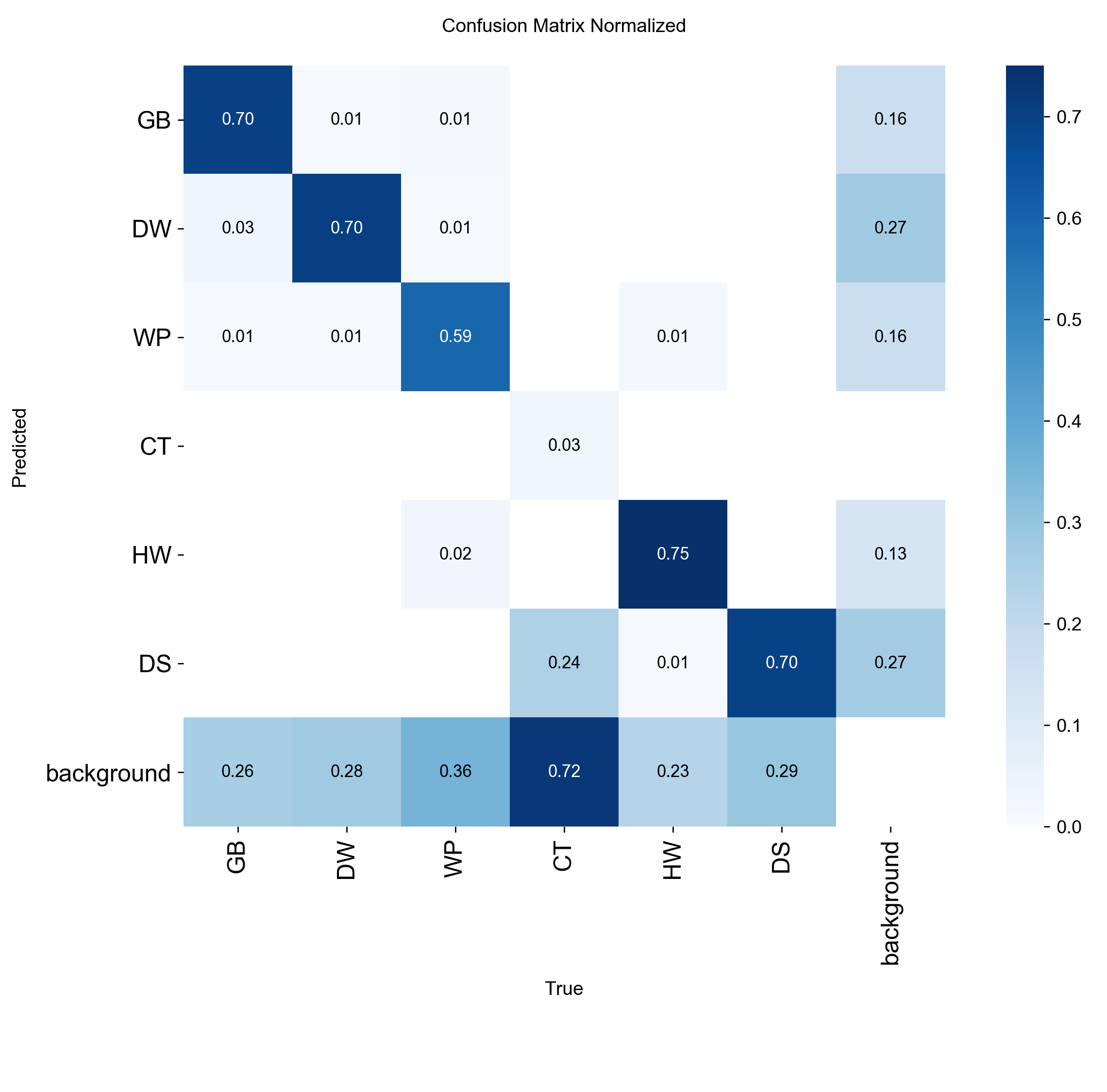
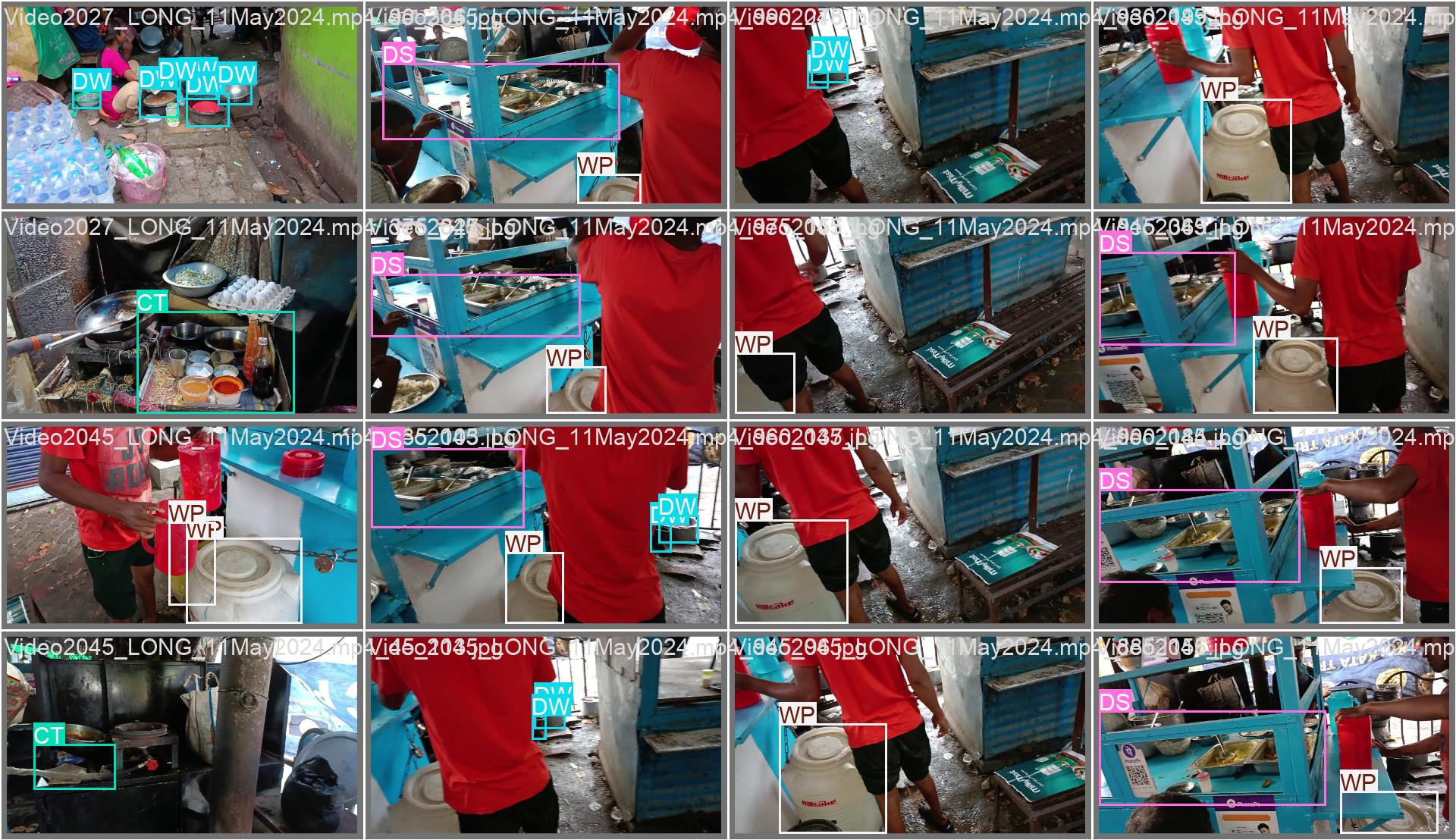
Counter top (CT)

A/Prof Klaus Ackermann
Department of Econometrics and Business Statistics, Melbourne, Monash University, Australia
A/Prof Denni Tommasi
Department of Economics, Bologna, University of Bologna, Italy
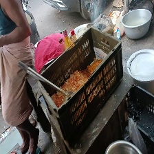
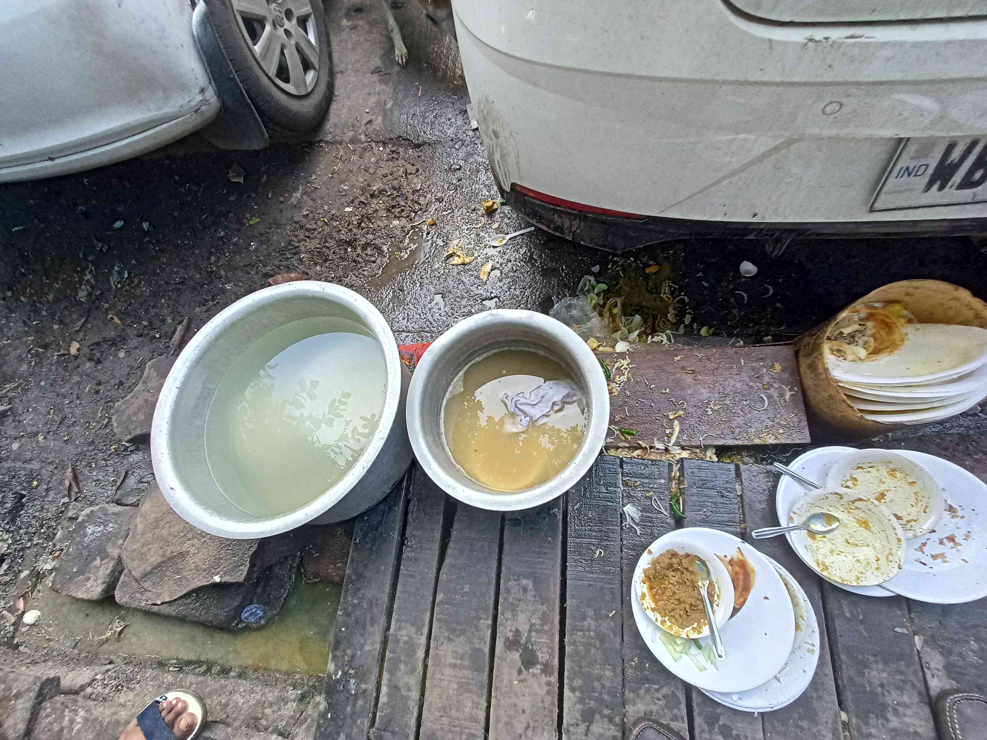
Street food is a major source of employment and an important food supply in many developing countries, but it is also often associated with significant food safety concerns.
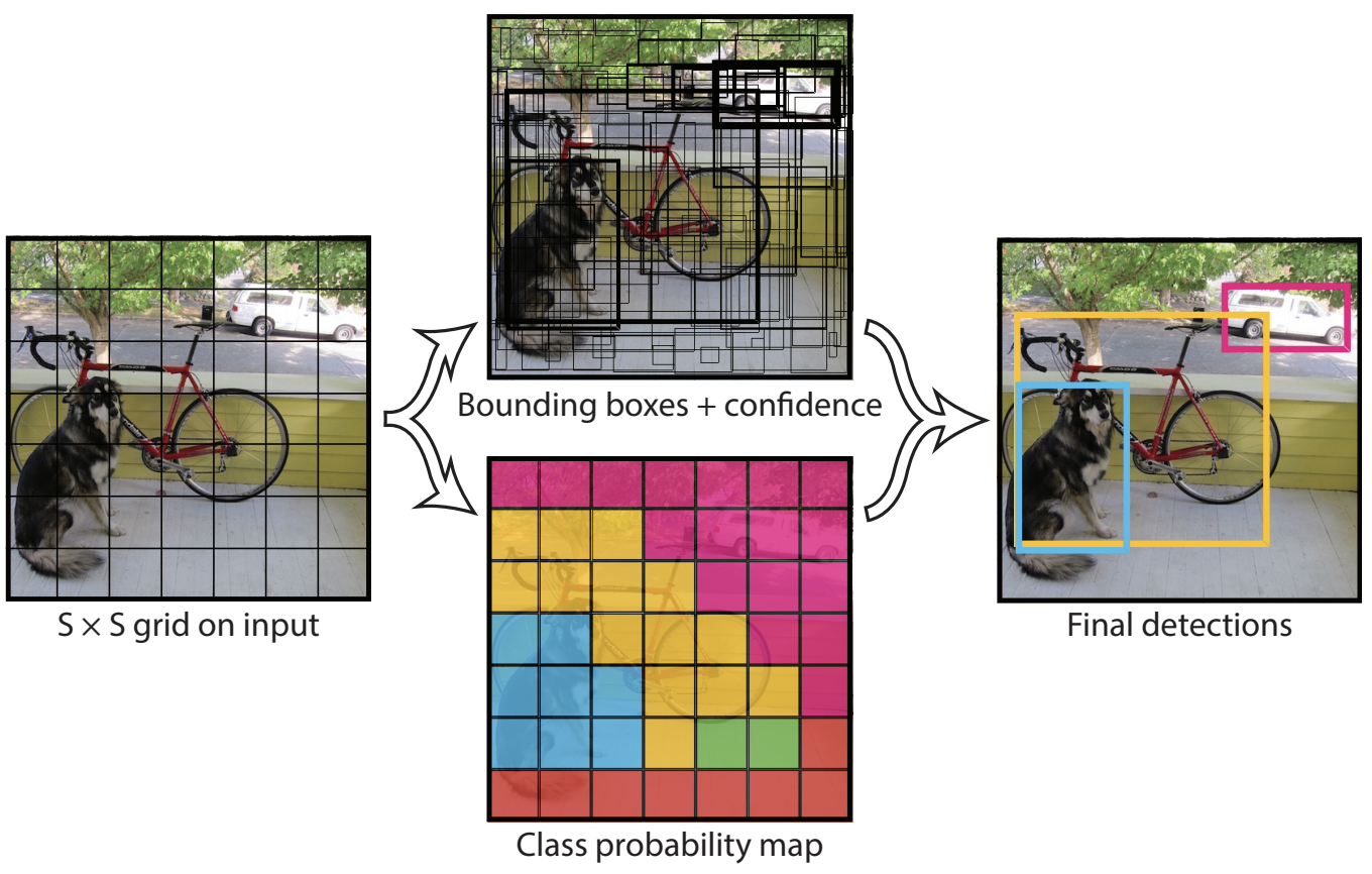
For each selected frame F_t, a pre-trained YOLOv10 model is applied to detect and localize objects in each frame:
\{(c_k, p_k, \mathbf{b}_k)\}_{k=1}^{K},
where c_k is the class label, p_k \in [0,1] is the confidence score, and \mathbf{b}_k = [x, y, w, h] denotes the bounding box (center coordinates and size). Here, K is the total number of detected objects in the frame.
An object is selected if p_k \ge \tau_{\text{od}}.
For each retained detection, an object crop C_k is extracted from the frame for further processing.
Counter top (CT)
Food displayed area (DS)
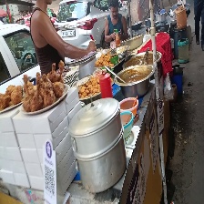
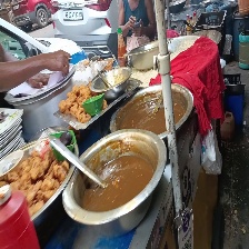
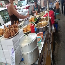
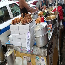
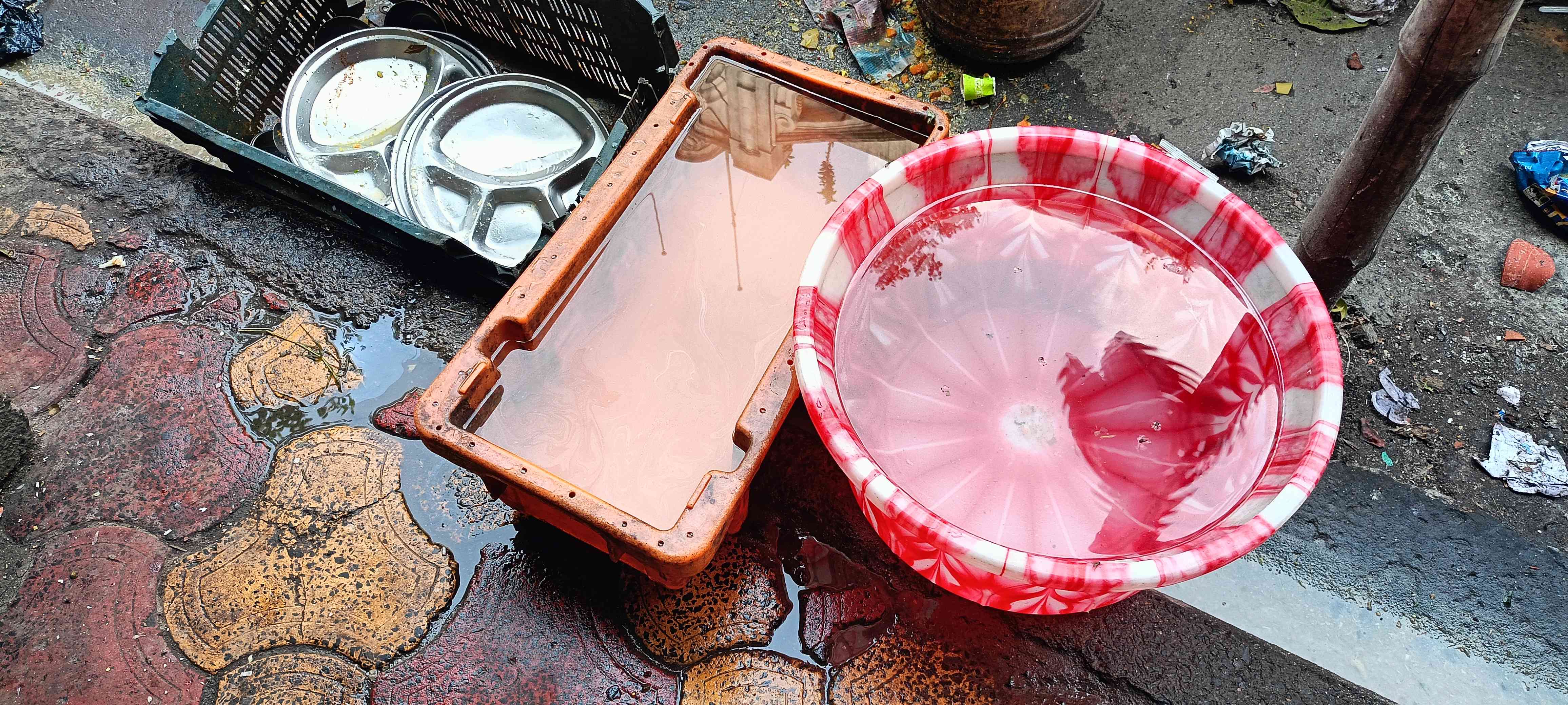
Dish-washing area (DW)
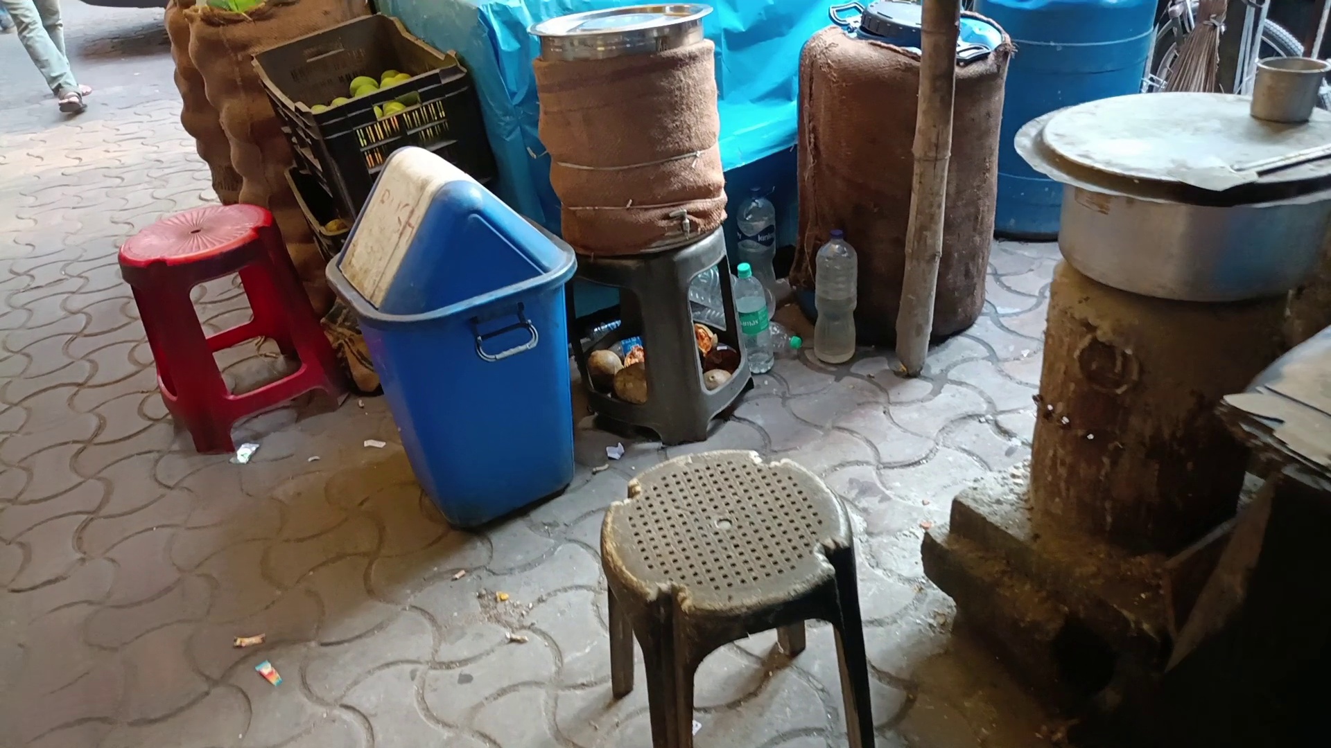
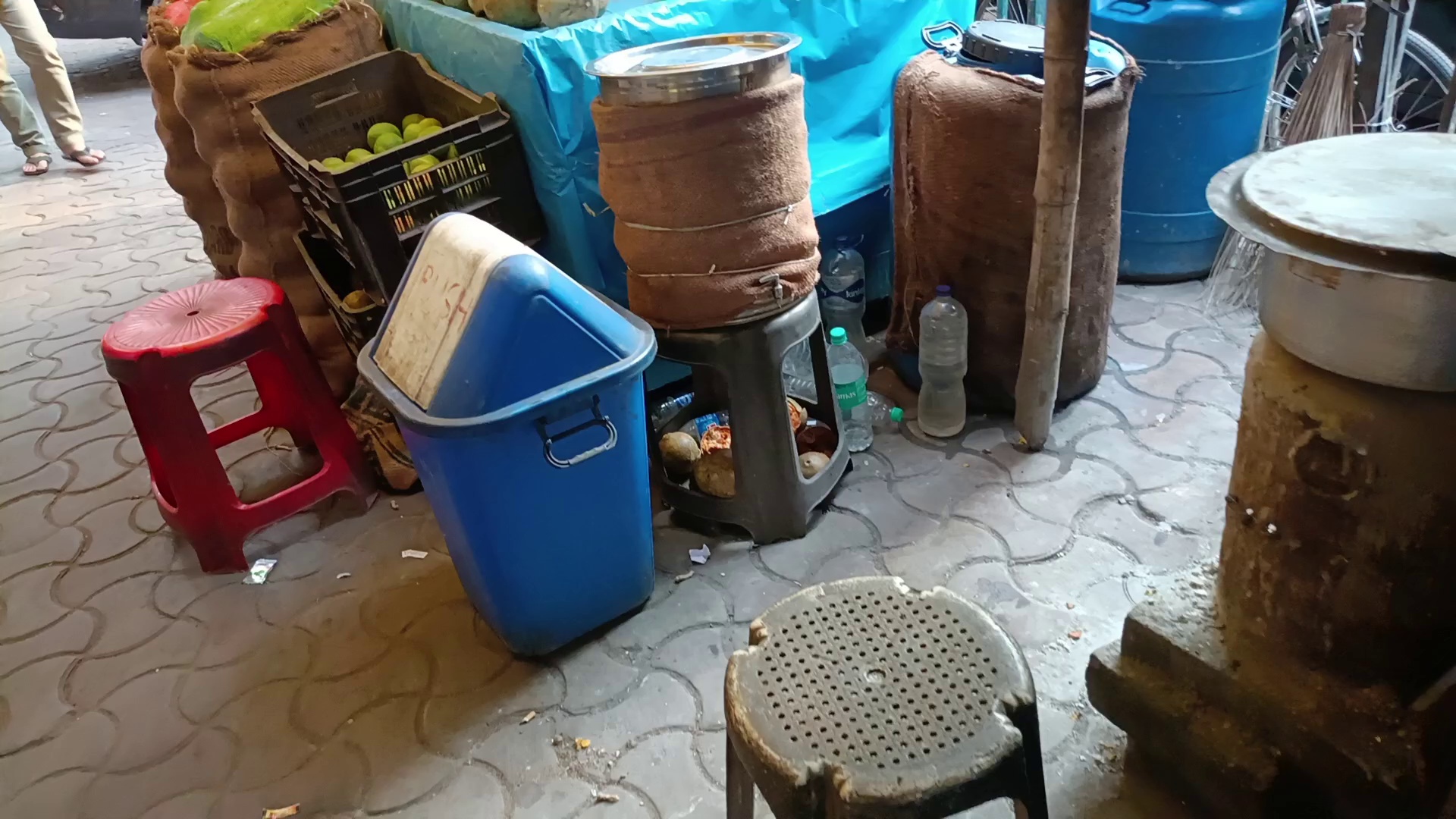
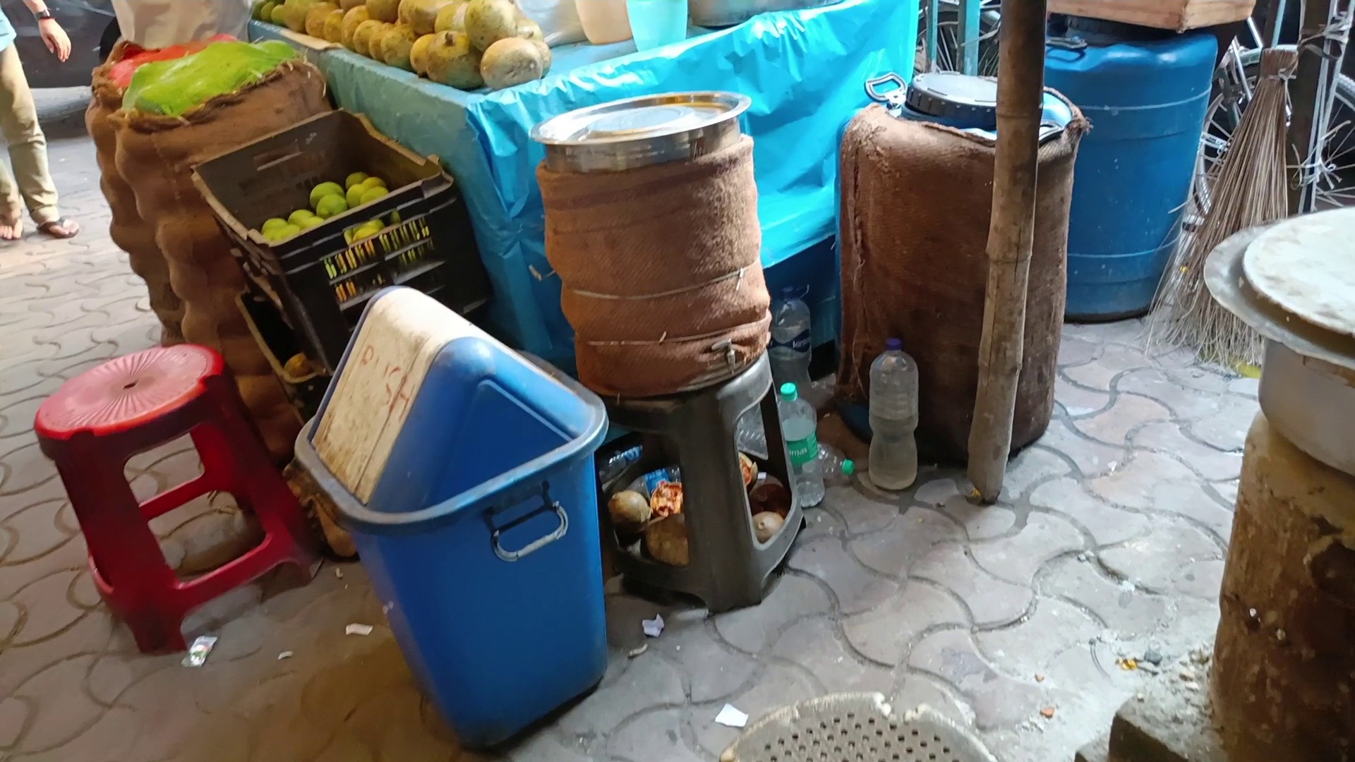
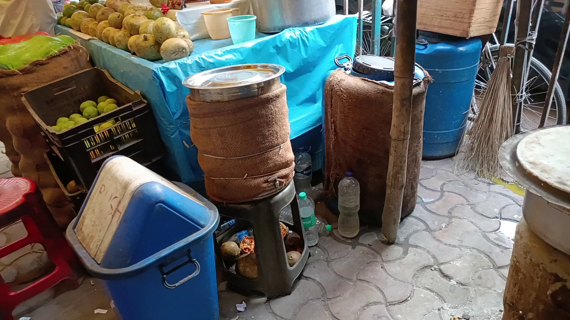
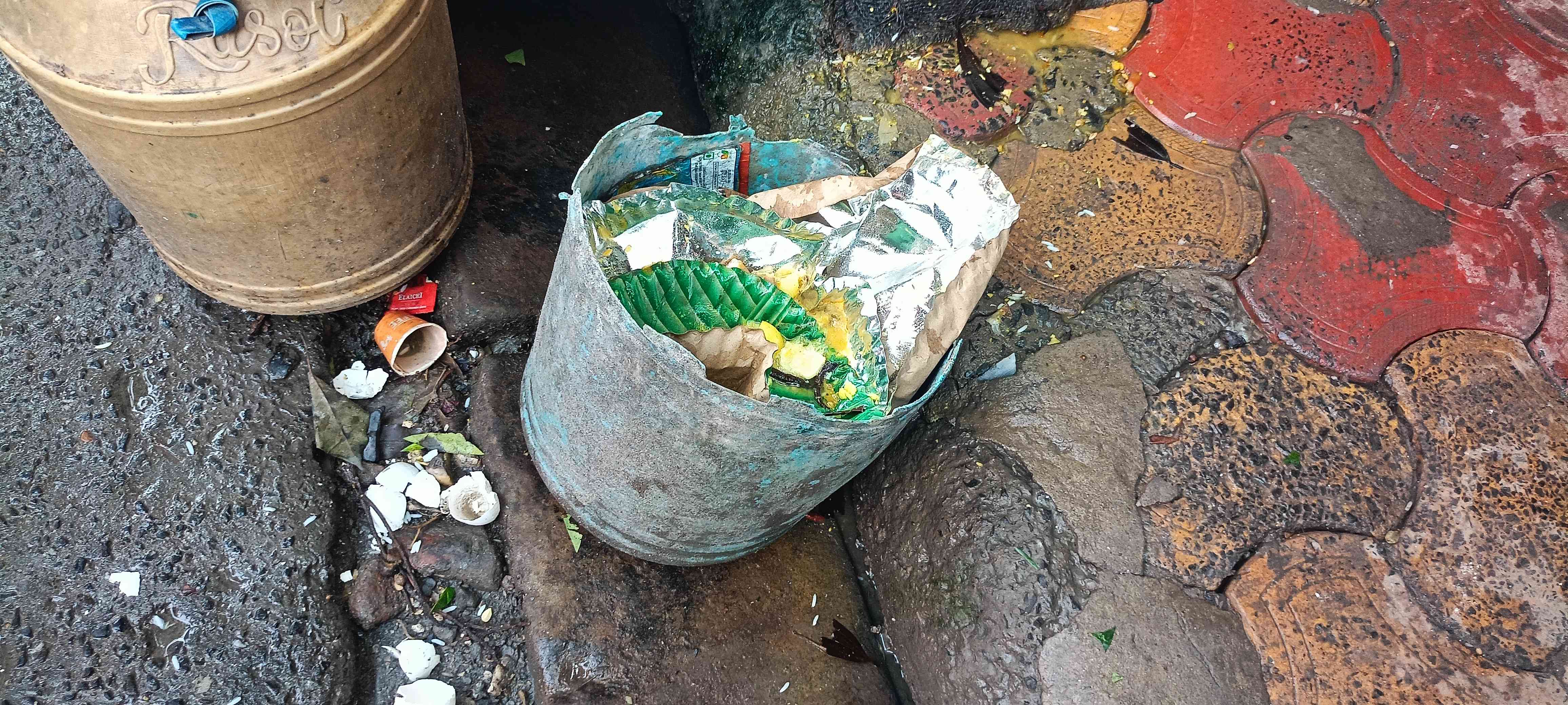
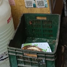
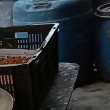
Garbage bin (GB)
Hand washing facility (HW)
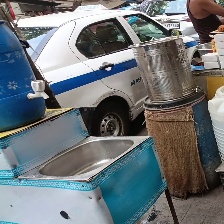
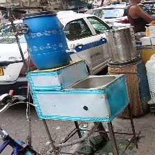
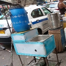
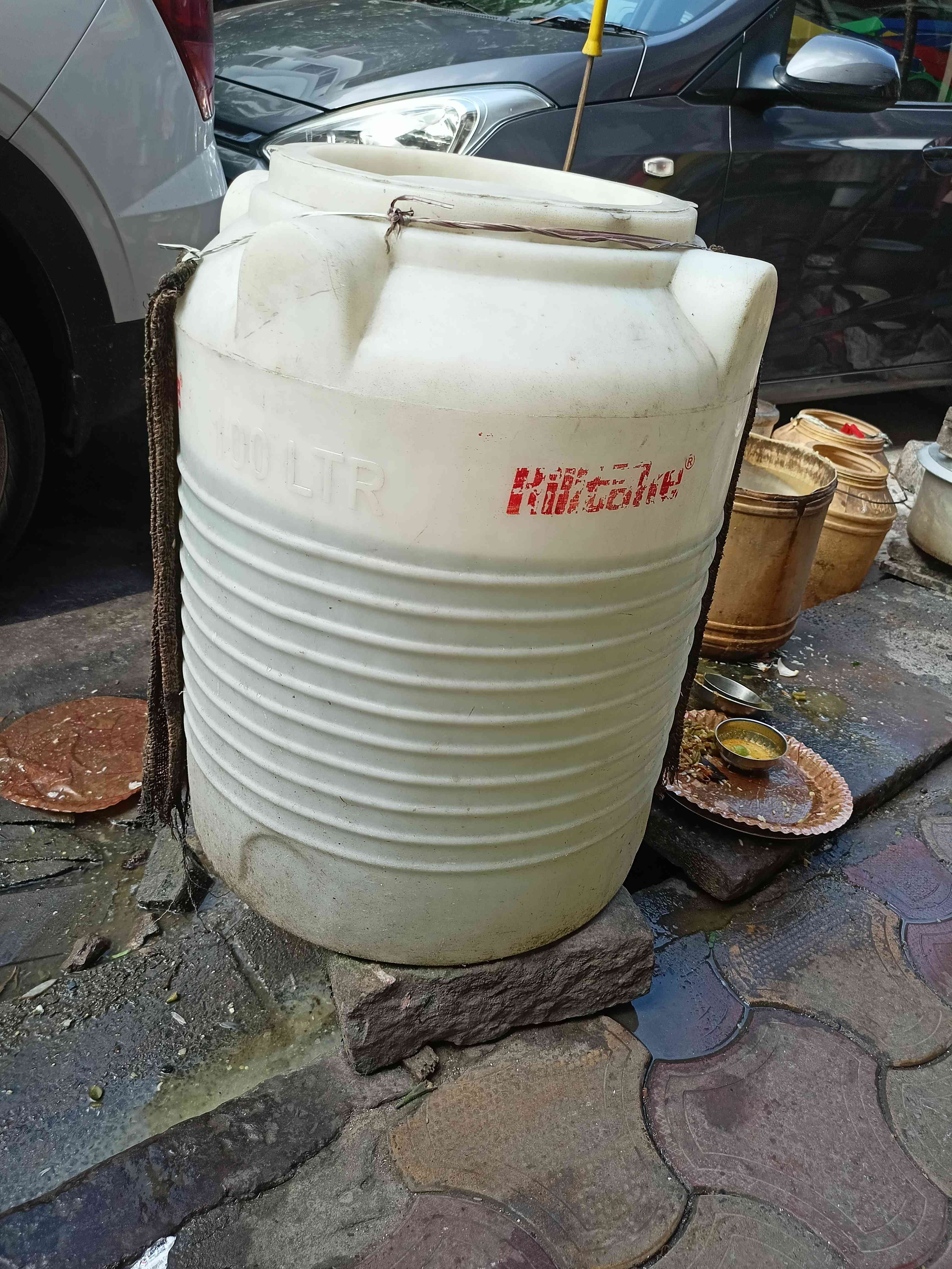
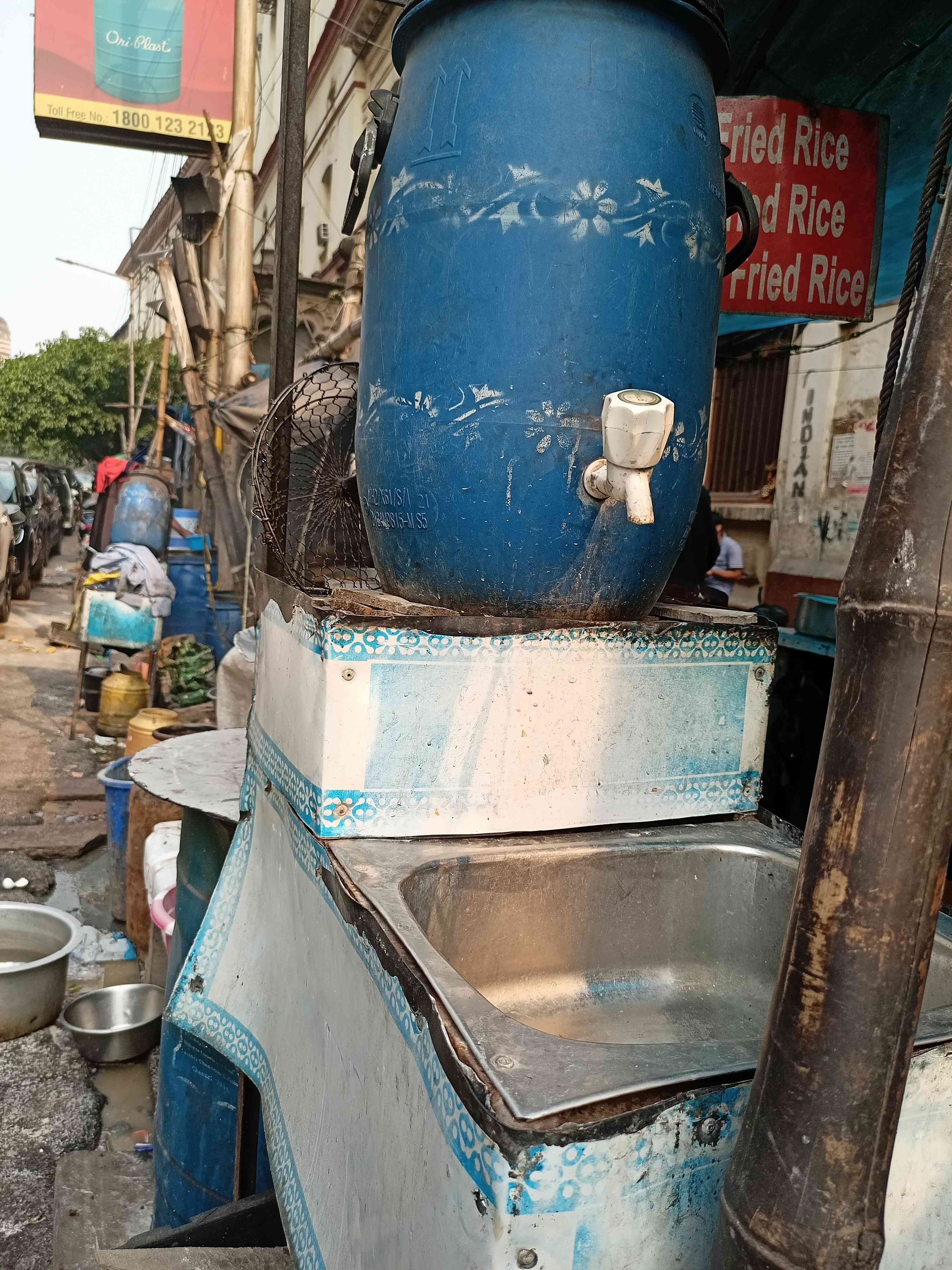
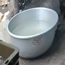
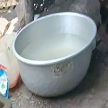
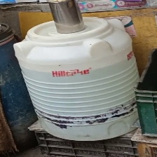
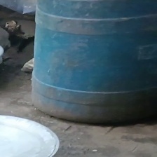
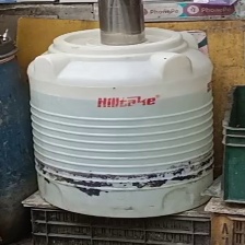
Water storage tank (WP)
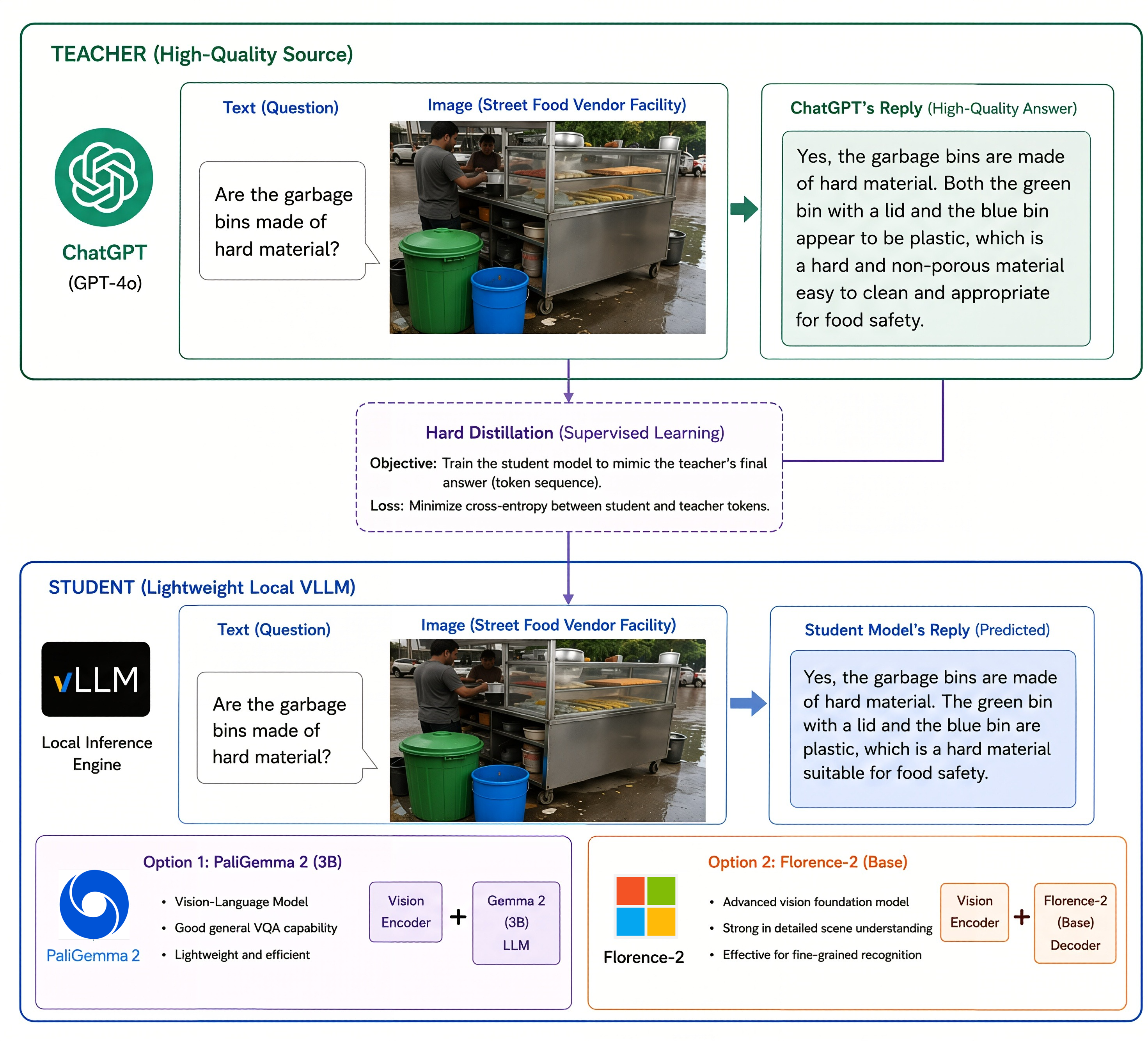
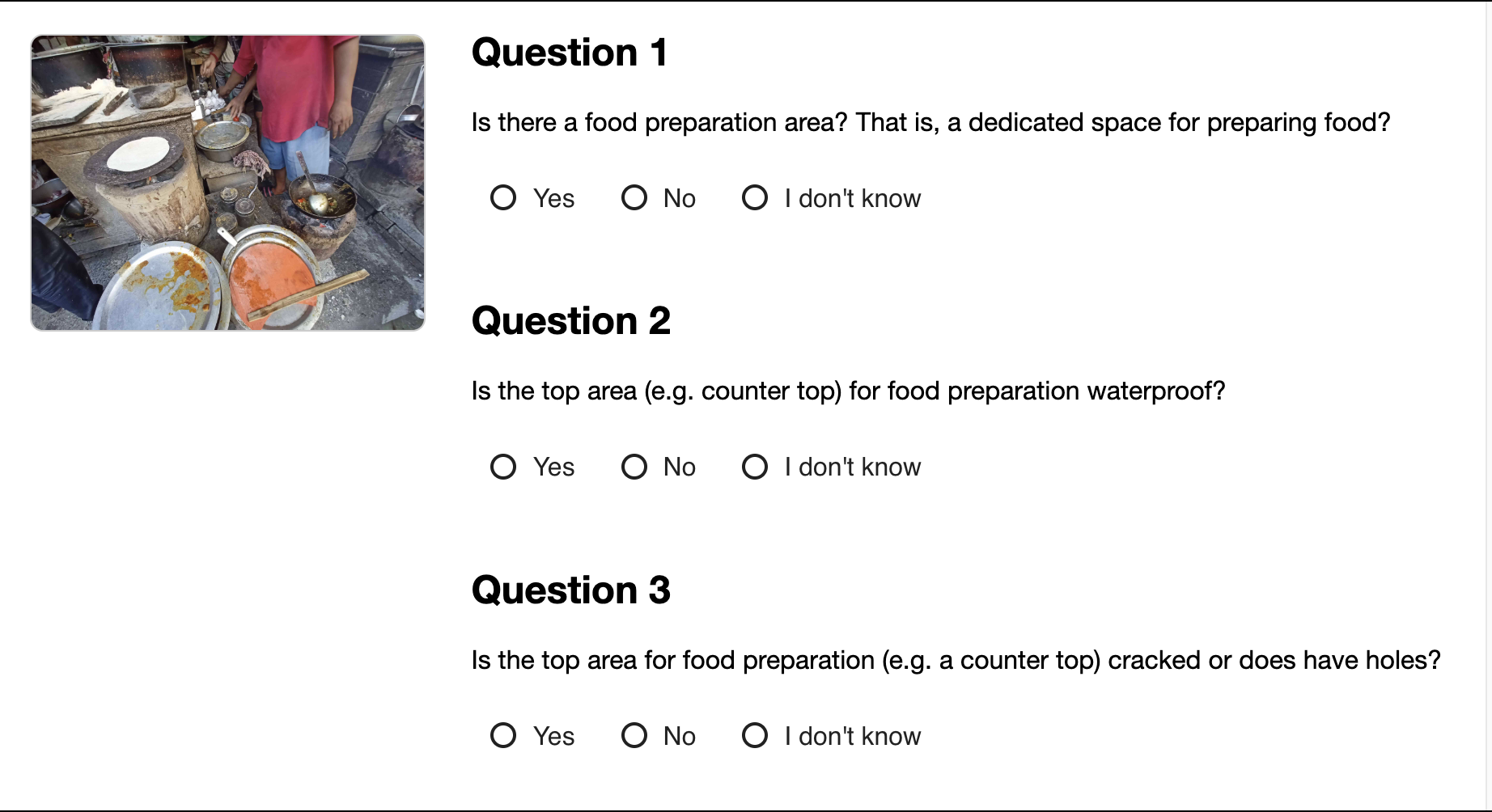
Class-specific questionnaires + corresponding images → ChatGPT-4o
Text prompt:
(1) Are the garbage bins made of hard material? E.g. metal, hard plastic? Answer type- Yes/No/Unknown
(2) Do the garbage bins have a smooth top area? Answer type- Yes/No/Unknown
(3) Are there animals/insects in or around the garbage bins? Answer type- Yes/No/Unknown
(4) Does the area around the garbage bins have standing water? Answer type- Yes/No/Unknown
(5) Are birds, insects, rodents or other animals present at the stall? Answer type- Yes/No/Unknown
Answer the questions above and return **JSON Lines**. Each line must contain the keys [qnum, short_ans, explanation].
Answers:
{"qnum":1,"short_ans":"yes","explanation":"The garbage bin appears to be a hard-material crate, likely plastic, rather than a flexible plastic bag or similar material."}
{"qnum":2,"short_ans":"no","explanation":"There are no visible cracks or holes in the garbage bin; the crate structure appears intact."}
{"qnum":3,"short_ans":"no","explanation":"There are no visible animals or insects in or around the garbage bin."}
{"qnum":4,"short_ans":"no","explanation":"There is no visible standing water around the garbage bin; the surrounding area appears dry."}
{"qnum":5,"short_ans":"no","explanation":"There are no visible animals or insects at the stall."}
Image:
Patchification (ViT) — Dosovitskiy et al. (2020), An Image is Worth 16×16 Words: Transformers for Image Recognition at Scale.
An example of attention matrix visualization — Vaswani, Ashish, et al. (2017), Attention Is All You Need.
![]()
An example of transformer block — Dosovitskiy et al. (2020), An Image is Worth 16×16 Words: Transformers for Image Recognition at Scale.
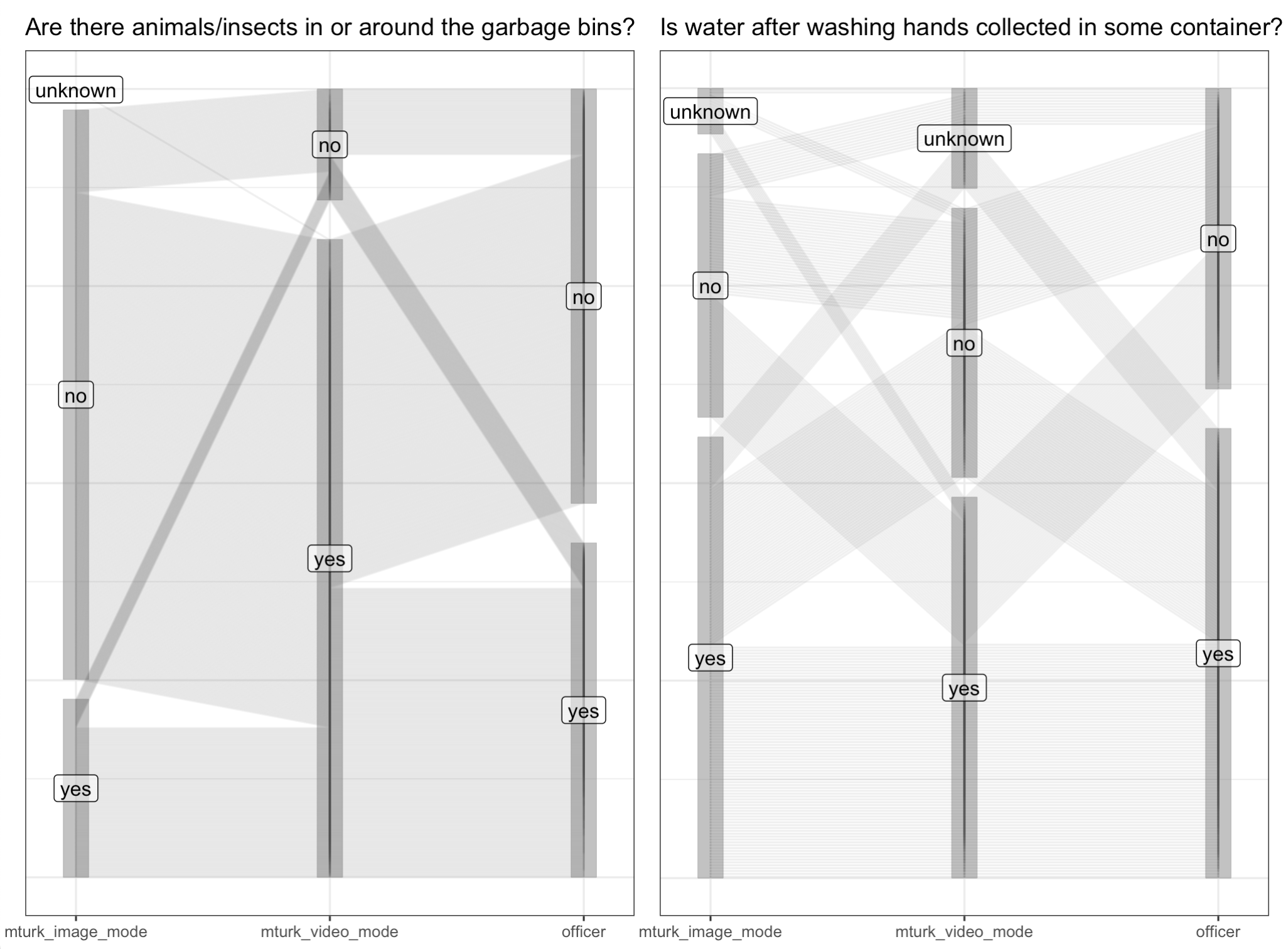
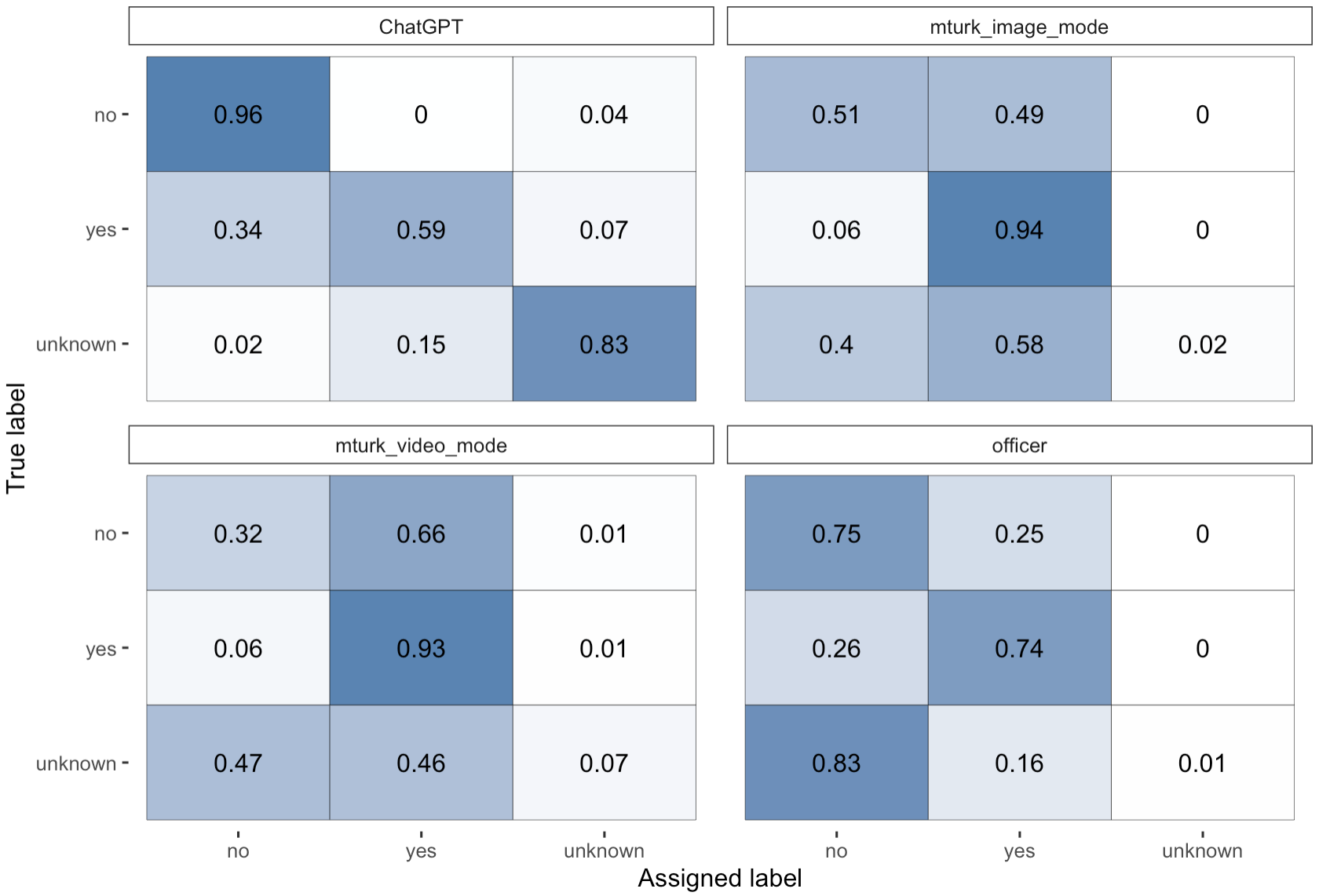
Neither ChatGPT nor officer annotations can be treated as absolute ground truth, as both contain inevitable errors. One effective way to reduce this noise is to collect additional annotations from diverse sources.
We conduct two human-subject experiments on Amazon Mechanical Turk (MTurk): one based on images and another based on short video clips, covering different classes of facilities.
Image study
Video study
Worker qualification criteria
For the animal/insect task, video-based annotations show a relatively high agreement rate with officers. In contrast, for the water collection task, the agreement between video-based annotations and officers is much lower, while image-based annotations achieve a comparatively higher agreement rate.
We define each item as a combination of vendor ID + video recording date + question.
We treat MTurk (image mode), MTurk (video mode), officer and ChatGPT as raters (distilled models are excluded).
The response space is: \{\text{yes}, \text{no}, \text{unknown}\} with \hat{\boldsymbol{\pi}} = (0.323, 0.606, 0.071).
| Rater | Agreement rate with estimated truth |
|---|---|
| ChatGPT mode | 0.852 |
| MTurk (image) | 0.824 |
| Officer | 0.737 |
| MTurk (video) | 0.709 |
| Florence-2 mode | 0.672 |
| PaliGemma mode | 0.663 |
tengmcing